Question

考虑从（-inf，inf）到[0,1]的非递减surjective（到）函数的集合。（典型的CDF s满足此属性。）换句话说，对于任何实数x，0 <= f（x）<= 1。 logistic function可能是最着名的例子。

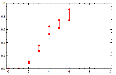
我们现在以x值列表的形式给出一些约束，并且对于每个x值，函数必须介于其间的一对y值。我们可以将其表示为{x，ymin，ymax}三元组列表，例如

constraints = {{0, 0, 0}, {1, 0.00311936, 0.00416369}, {2, 0.0847077, 0.109064}, 
 {3, 0.272142, 0.354692}, {4, 0.53198, 0.646113}, {5, 0.623413, 0.743102}, 
 {6, 0.744714, 0.905966}}

图形上看起来像这样：

constraints on a cdf http://yootles.com/outbox/cdffit1.png

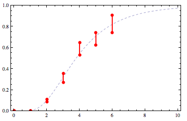
我们现在寻求一条尊重这些约束的曲线。例如：

fitted cdf http://yootles.com/outbox/cdffit2.png

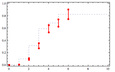
让我们首先尝试通过约束的中点进行简单插值：

mids = ({#1, Mean[{#2,#3}]}&) @@@ constraints
f = Interpolation[mids, InterpolationOrder->0]

Plotted，f看起来像这样：

interpolated cdf http://yootles.com/outbox/cdffit3.png

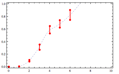
这个功能不是满足的。此外，我们希望它更顺畅。我们可以增加插值顺序，但现在它违反了其范围为[0,1]的约束：

interpolated cdf with higher interpolation order http://yootles.com/outbox/cdffit4.png

然后，目标是找到满足约束条件的smoothest function：

非递减。
当x接近负无穷大时倾向于0，当x接近无穷大时倾向于1。
通过给定的y-error-bars列表。

我上面绘制的第一个例子似乎是一个很好的候选人，但是我使用Mathematica的FindFit函数假设lognormal CDF。这在这个具体示例中效果很好，但通常不需要满足约束的对数正态CDF。

Answer 1

我认为您没有指定足够的标准来使所需的CDF独一无二。

如果必须遵守的唯一标准是：

CDF必须“相当顺利”（见下文）
CDF必须不减少
CDF必须通过“错误栏”y间隔
CDF必须趋于0，因为x - > -无穷
CDF必须倾向于1，因为x - >无穷。

那么也许你可以使用Monotone Cubic Interpolation。这将给你一个C ^ 2（两次连续可微）的功能，与三次样条不同，在给定单调数据时保证单调。

这留下了一个问题，确切地说，您应该使用哪些数据来生成单调立方插值。如果取每个错误的中心点（平均值） bar，您是否保证结果数据点是单调的增加？如果没有，你可以做出一些任意选择来保证您选择的点是单调递增的（因为标准不会强制我们的解决方案是唯一的）。

现在该如何处理最后一个数据点？是否有保证的X. 是否大于约束数据集中的任何x？也许你可以再做一次随意选择方便并挑选一些非常大的X并将（X，1）作为最终数据点。

评论1：您的问题可分为2个子问题：

给定CDF必须通过的确切点（x_i，y_i），如何生成CDF？我怀疑有无限多种可能的解决方案，即使有无限平滑约束。
鉴于y-errorbars，你应该如何选择（x_i，y_i）？同样，有无限多种可能的解决方案。可能需要添加一些额外的标准来强制进行独特的选择。其他标准也可能使问题比现在更难。

评论2：这是一种使用单调三次插值并满足标准4和5的方法：

单调三次插值（我们称之为f）映射 R - ＆gt;的 - [R 即可。

让CDF(x) = exp(-exp(f(x)))。然后是CDF: R --> (0,1)。如果我们能找到合适的f，那么通过这种方式定义CDF，我们就可以满足标准4和5。

要查找f，请使用转化(x_0,y_0),...,(x_n,y_n)，xhat_i = x_i转换CDF约束yhat_i = log(-log(y_i))。这是CDF转换的反转。如果y_i增加，则yhat_i正在减少。

现在将单调三次插值应用于（x_hat，y_hat）数据点以生成f。最后，定义CDF(x) = exp(-exp(f(x)))。这将是 R - >的单调递增函数。（0,1），它通过点（x_i，y_i）。

我认为，这符合所有标准2--5。标准1有点满意，但肯定可以存在更平滑的解决方案。

Answer 2

我找到了一种解决方案，可以为各种输入提供合理的结果。我首先拟合一个模型 - 一次到约束的低端，再一次到高端。我将这两个拟合函数的平均值称为“理想函数”。我使用这个理想函数来推断约束结束的左侧和右侧，以及在约束中的任何间隙之间进行插值。我以规则的间隔计算理想函数的值，包括所有约束，从左边的函数几乎为零，到右边的函数几乎为零。在约束条件下，我会根据需要剪切这些值以满足约束条件。最后，我构造了一个遍历这些值的插值函数。

我的Mathematica实施如下首先，一对辅助函数：

(* Distance from x to the nearest member of list l. *)
listdist[x_, l_List] := Min[Abs[x - #] & /@ l]

(* Return a value x for the variable var such that expr/.var->x is at least (or
   at most, if dir is -1) t. *)
invertish[expr_, var_, t_, dir_:1] := Module[{x = dir},
  While[dir*(expr /. var -> x) < dir*t, x *= 2];
  x]

这是主要功能：

(* Return a non-decreasing interpolating function that maps from the
   reals to [0,1] and that is as close as possible to expr[var] without
   violating the given constraints (a list of {x,ymin,ymax} triples).
   The model, expr, will have free parameters, params, so first do a
   model fit to choose the parameters to satisfy the constraints as well
   as possible. *)
cfit[constraints_, expr_, params_, var_] := 
Block[{xlist,bots,tops,loparams,hiparams,lofit,hifit,xmin,xmax,gap,aug,bests},
  xlist = First /@ constraints;
  bots = Most /@ constraints; (* bottom points of the constraints *)
  tops = constraints /. {x_, _, ymax_} -> {x, ymax};
  (* fit a model to the lower bounds of the constraints, and 
     to the upper bounds *)
  loparams = FindFit[bots, expr, params, var];
  hiparams = FindFit[tops, expr, params, var];
  lofit[z_] = (expr /. loparams /. var -> z);
  hifit[z_] = (expr /. hiparams /. var -> z);
  (* find x-values where the fitted function is very close to 0 and to 1 *)
  {xmin, xmax} = {
    Min@Append[xlist, invertish[expr /. hiparams, var, 10^-6, -1]],
    Max@Append[xlist, invertish[expr /. loparams, var, 1-10^-6]]};
  (* the smallest gap between x-values in constraints *)
  gap = Min[(#2 - #1 &) @@@ Partition[Sort[xlist], 2, 1]];
  (* augment the constraints to fill in any gaps and extrapolate so there are 
     constraints everywhere from where the function is almost 0 to where it's 
     almost 1 *)
  aug = SortBy[Join[constraints, Select[Table[{x, lofit[x], hifit[x]}, 
                                              {x, xmin,xmax, gap}], 
                                        listdist[#[[1]],xlist]>gap&]], First];
  (* pick a y-value from each constraint that is as close as possible to 
     the mean of lofit and hifit *)
  bests = ({#1, Clip[(lofit[#1] + hifit[#1])/2, {#2, #3}]} &) @@@ aug;
  Interpolation[bests, InterpolationOrder -> 3]]

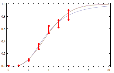
例如，我们可以适应对数正态，正态或逻辑函数：

g1 = cfit[constraints, CDF[LogNormalDistribution[mu,sigma], z], {mu,sigma}, z]
g2 = cfit[constraints, CDF[NormalDistribution[mu,sigma], z], {mu,sigma}, z]
g3 = cfit[constraints, 1/(1 + c*Exp[-k*z]), {c,k}, z]

以下是我原始示例约束列表中的内容：

constrained fit to lognormal, normal, and logistic function http://yootles.com/outbox/cdffit5.png

正态和逻辑几乎相互叠加，对数正态是蓝色曲线。

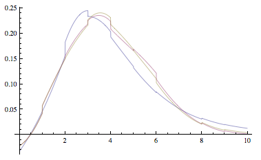
这些并不完美。特别是，它们并不是单调的。这是衍生品的图表：

Plot[{g1'[x], g2'[x], g3'[x]}, {x, 0, 10}]

the derivatives of the fitted functions http://yootles.com/outbox/cdffit6.png

这表明一些缺乏平滑性以及零附近的轻微非单调性。我欢迎对此解决方案进行改进！

Answer 3

您可以尝试通过中点适合Bezier curve。具体来说，我认为你想要C2 continuous曲线。

曲线拟合：找到满足约束列表的最流畅的函数

3 个答案: