如何在Mathematica中绘制单位单形上定义的函数？

Question

我正在尝试在单位单纯形中定义的 Mathematica 中绘制一个函数。举一个随机的例子，假设我想在所有x1，x2，x3上绘制sin（x1 * x2 * x3），使得x1，x2，x3＆gt; = 0和x1 + x2 + x3 = 1。 有没有一种巧妙的方式这样做，除了显而易见的写作方式

Plot3D[If[x+y<=1,Sin[x y(1-x-y)]],{x,0,1},{y,0,1}]

？

理想情况下，我想要的是在单纯形图上绘制仅的方法。我发现网站http://octavia.zoology.washington.edu/Mathematica/有一个旧包，但它不适用于我最新版本的 Mathematica 。

Answer 1

如果你想得到你所链接的那个包中的对称外观图，你需要弄清楚将单纯形放入x / y平面的旋转矩阵。您可以在下面使用此功能。这有点长，因为我在计算中留下了解单面中心。具有讽刺意味的是，4d单形图的转换要简单得多。修改e变量以获得不同的保证金

simplexPlot[func_, plotFunc_] := 
 Module[{A, B, p2r, r2p, p1, p2, p3, e, x1, x2, w, h, marg, y1, y2, 
   valid},
  A = Sqrt[2/3] {Cos[#], Sin[#], Sqrt[1/2]} & /@ 
     Table[Pi/2 + 2 Pi/3 + 2 k Pi/3, {k, 0, 2}] // Transpose;
  B = Inverse[A];

  (* map 3d probability vector into 2d vector *)
  p2r[{x_, y_, z_}] := Most[A.{x, y, z}];

  (* map 2d vector in 3d probability vector *)
  r2p[{u_, v_}] := B.{u, v, Sqrt[1/3]};

  (* Bounds to center the simplex *)
  {p1, p2, p3} = Transpose[A];

  (* extra padding to use *)
  e = 1/20;

  x1 = First[p1] - e/2;
  x2 = First[p2] + e/2;
  w = x2 - x1;
  h = p3[[2]] - p2[[2]];
  marg = (w - h + e)/2;
  y1 = p2[[2]] - marg;
  y2 = p3[[2]] + marg;

  valid = 
   Function[{x, y}, Min[r2p[{x, y}]] >= 0 && Max[r2p[{x, y}]] <= 1];
  plotFunc[func @@ r2p[{x, y}], {x, x1, x2}, {y, y1, y2}, 
   RegionFunction -> valid]
  ]

以下是如何使用它

simplexPlot[Sin[#1 #2 #3] &, Plot3D]

http://yaroslavvb.com/upload/save/simplex-plot1.png

simplexPlot[Sin[#1 #2 #3] &, DensityPlot]

http://yaroslavvb.com/upload/save/simplex-plot2.png

如果要在原始坐标系中查看域，可以将绘图旋转回单面

t = AffineTransform[{{{-(1/Sqrt[2]), -(1/Sqrt[6]), 1/Sqrt[3]}, {1/
      Sqrt[2], -(1/Sqrt[6]), 1/Sqrt[3]}, {0, Sqrt[2/3], 1/Sqrt[
      3]}}, {1/3, 1/3, 1/3}}];
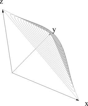
graphics = simplexPlot[5 Sin[#1 #2 #3] &, Plot3D];
shape = Cases[graphics, _GraphicsComplex];
Graphics3D[{Opacity[.5], GeometricTransformation[shape, t]}, 
 Axes -> True]

http://yaroslavvb.com/upload/save/raster2.png

这是另一个单纯形图，使用here和MeshFunctions->{#3&}中的传统三维轴，完整代码here

http://yaroslavvb.com/upload/save/simplex.png

Answer 2

尝试：

Plot3D[Sin[x y (1 - x - y)], {x, 0, 1}, {y, 0, 1 - x}]

但您也可以使用Piecewise和RegionFunction：

Plot3D[Piecewise[{{Sin[x y (1 - x - y)], 
    x >= 0 && y >= 0 && x + y <= 1}}], {x, 0, 1}, {y, 0, 1}, 
 RegionFunction -> Function[{x, y}, x + y <= 1]]