еҰӮдҪ•з»ҳеҲ¶й«ҳж–Ҝжңҙзҙ иҙқеҸ¶ж–ҜеҲҶзұ»еҷЁзҡ„еҶізӯ–иҫ№з•Ңпјҹ
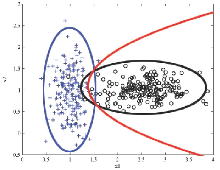
жҲ‘дҪҝз”ЁдёӢйқўзҡ„зҺ©е…·ж•°жҚ®йӣҶпјҲзұ»жҲҗе‘ҳеҸҳйҮҸпјҶamp; 2зү№еҫҒпјүжқҘеә”з”Ёй«ҳж–Ҝжңҙзҙ иҙқеҸ¶ж–ҜжЁЎеһӢ并з»ҳеҲ¶зү№е®ҡдәҺзұ»зҡ„еҸҢеҸҳйҮҸжӯЈжҖҒеҲҶеёғзҡ„иҪ®е»“гҖӮ
еҰӮдҪ•дёәеҶізӯ–иҫ№з•Ңж·»еҠ дёҖжқЎзәҝеҲ°дёӢйқўзҡ„еӣҫпјҹ пјҲжҜ”еҰӮиҝҷйҮҢпјҡhttps://alliance.seas.upenn.edu/~cis520/dynamic/2016/wiki/uploads/Lectures/2class_gauss_NB.jpgпјү
# Packages
library(klaR)
library(MASS)

# Data
d <- structure(list(y = structure(c(1L, 1L, 1L, 1L, 2L, 2L, 2L, 2L, 2L, 1L), .Label = c("0", "1"), class = "factor"), x1 = c(2, 2.8, 1.5, 2.1, 5.5, 8, 6.9, 8.5, 2.5, 7.7), x2 = c(1.5, 1.2, 1, 1, 4, 4.8, 4.5, 5.5, 2, 3.5)), .Names = c("y", "x1", "x2"), row.names = c(NA, -10L), class = "data.frame")

# Naive Bayes Model
mN <- NaiveBayes(y ~ x1+x2, data = d)

# Data

# Class 1
m1 <- mean(d[which(d$y==1),]$x1)
m2 <- mean(d[which(d$y==1),]$x2)
mu1_2 <- c(m1,m2)  # Mean
sd1 <- sd(d[which(d$y==1),]$x1)
sd2 <- sd(d[which(d$y==1),]$x2)
Sigma1_2 <- matrix(c(sd1, 0, 0, sd2), 2)  # Covariance matrix
bivn1_2 <- mvrnorm(5000, mu = mu1_2, Sigma = Sigma1_2 )  # from Mass package: Simulate bivariate normal PDF
bivn1_2.kde <- kde2d(bivn1_2[,1], bivn1_2[,2], n = 50)   # from MASS package: Calculate kernel density estimate


# Class 0
m3 <- mean(d[which(d$y==0),]$x1)
m4 <- mean(d[which(d$y==0),]$x2)
mu3_4 <- c(m3,m4)  # Mean
sd3 <- sd(d[which(d$y==0),]$x1)
sd4 <- sd(d[which(d$y==0),]$x2)
Sigma3_4 <- matrix(c(sd3, 0, 0, sd4), 2)  # Covariance matrix
bivn3_4 <- mvrnorm(5000, mu = mu3_4, Sigma = Sigma3_4 )  # from Mass package: Simulate bivariate normal PDF
bivn3_4.kde <- kde2d(bivn3_4[,1], bivn3_4[,2], n = 50)   # from MASS package: Calculate kernel density estimate


# Plot
plot(x= d$x1, y=d$x2, xlim=c(-1,10), ylim=c(-1,10), col=d$y, pch=19, cex=2, ylab="x2", xlab="x1")
contour(bivn1_2.kde, add = TRUE, col="darkgrey")     # from base graphics package
contour(bivn3_4.kde, add = TRUE, col="darkgrey") # from base graphics package
text(labels = "Class 1",x = 8, y=7, col="grey")
text(labels = "Class 0",x = 0, y=4, col="grey")

0 дёӘзӯ”жЎҲ:
жІЎжңүзӯ”жЎҲ
зӣёе…ій—®йўҳ
- е®һзҺ°й«ҳж–Ҝжңҙзҙ иҙқеҸ¶ж–Ҝ
- еҶізӯ–ж ‘дёҺжңҙзҙ иҙқеҸ¶ж–ҜеҲҶзұ»еҷЁ
- й«ҳж–Ҝжңҙзҙ иҙқеҸ¶ж–ҜеҲҶзұ»
- жңҙзҙ иҙқеҸ¶ж–ҜеҲҶзұ»еҷЁ
- SciKit-learn - и®ӯз»ғй«ҳж–Ҝжңҙзҙ иҙқеҸ¶ж–ҜеҲҶзұ»еҷЁ
- еҰӮдҪ•з»ҳеҲ¶й«ҳж–Ҝжңҙзҙ иҙқеҸ¶ж–ҜеҲҶзұ»еҷЁзҡ„еҶізӯ–иҫ№з•Ңпјҹ
- еңЁж•°еӯ—еҲҶзұ»ж•°жҚ®дёҠе®һзҺ°жңҙзҙ иҙқеҸ¶ж–Ҝй«ҳж–ҜеҲҶзұ»еҷЁ
- жңҙзҙ иҙқеҸ¶ж–Ҝж··еҗҲз®—жі•пјҲй«ҳж–Ҝе’ҢеҲҶзұ»еҷЁпјү
- жңҖйҮҚиҰҒзҡ„зү№еҫҒй«ҳж–Ҝжңҙзҙ иҙқеҸ¶ж–ҜеҲҶзұ»еҷЁpython sklearn
- д»Җд№ҲжҳҜPythonпјҲй«ҳж–Ҝжңҙзҙ иҙқеҸ¶ж–Ҝпјүдёӯзҡ„еҲҶзұ»еҷЁпјҹ
жңҖж–°й—®йўҳ
- жҲ‘еҶҷдәҶиҝҷж®өд»Јз ҒпјҢдҪҶжҲ‘ж— жі•зҗҶи§ЈжҲ‘зҡ„й”ҷиҜҜ
- жҲ‘ж— жі•д»ҺдёҖдёӘд»Јз Ғе®һдҫӢзҡ„еҲ—иЎЁдёӯеҲ йҷӨ None еҖјпјҢдҪҶжҲ‘еҸҜд»ҘеңЁеҸҰдёҖдёӘе®һдҫӢдёӯгҖӮдёәд»Җд№Ҳе®ғйҖӮз”ЁдәҺдёҖдёӘз»ҶеҲҶеёӮеңәиҖҢдёҚйҖӮз”ЁдәҺеҸҰдёҖдёӘз»ҶеҲҶеёӮеңәпјҹ
- жҳҜеҗҰжңүеҸҜиғҪдҪҝ loadstring дёҚеҸҜиғҪзӯүдәҺжү“еҚ°пјҹеҚўйҳҝ
- javaдёӯзҡ„random.expovariate()
- Appscript йҖҡиҝҮдјҡи®®еңЁ Google ж—ҘеҺҶдёӯеҸ‘йҖҒз”өеӯҗйӮ®д»¶е’ҢеҲӣе»әжҙ»еҠЁ
- дёәд»Җд№ҲжҲ‘зҡ„ Onclick з®ӯеӨҙеҠҹиғҪеңЁ React дёӯдёҚиө·дҪңз”Ёпјҹ
- еңЁжӯӨд»Јз ҒдёӯжҳҜеҗҰжңүдҪҝз”ЁвҖңthisвҖқзҡ„жӣҝд»Јж–№жі•пјҹ
- еңЁ SQL Server е’Ң PostgreSQL дёҠжҹҘиҜўпјҢжҲ‘еҰӮдҪ•д»Һ第дёҖдёӘиЎЁиҺ·еҫ—第дәҢдёӘиЎЁзҡ„еҸҜи§ҶеҢ–
- жҜҸеҚғдёӘж•°еӯ—еҫ—еҲ°
- жӣҙж–°дәҶеҹҺеёӮиҫ№з•Ң KML ж–Ү件зҡ„жқҘжәҗпјҹ