我正在尝试用Python中的1个隐藏层实现基本的XOR NN。我不是特别了解backprop算法,所以我一直坚持使用delta2并更新权重...帮助?
import numpy as np

def sigmoid(x):
    return 1.0 / (1.0 + np.exp(-x))

vec_sigmoid = np.vectorize(sigmoid)

theta1 = np.matrix(np.random.rand(3,3))
theta2 = np.matrix(np.random.rand(3,1))

def fit(x, y, theta1, theta2, learn_rate=.001):
    #forward pass
    layer1 = np.matrix(x, dtype='f')
    layer1 = np.c_[np.ones(1), layer1]
    layer2 = vec_sigmoid(layer1*theta1)
    layer3 = sigmoid(layer2*theta2)

    #backprop
    delta3 = y - layer3
    delta2 = (theta2*delta3) * np.multiply(layer2, 1 - layer2) #??

    #update weights
    theta2 += learn_rate * delta3 #??
    theta1 += learn_rate * delta2 #??

def train(X, Y):
    for _ in range(10000):
        for i in range(4):
            x = X[i]
            y = Y[i]
            fit(x, y, theta1, theta2)


X = [(0,0), (1,0), (0,1), (1,1)]
Y = [0, 1, 1, 0]
train(X, Y)
答案 0 :(得分:4)
好的,首先,这是修改后的代码,让你的工作。
#! /usr/bin/python

import numpy as np

def sigmoid(x):
    return 1.0 / (1.0 + np.exp(-x))

vec_sigmoid = np.vectorize(sigmoid)

# Binesh - just cleaning it up, so you can easily change the number of hiddens.
# Also, initializing with a heuristic from Yoshua Bengio.
# In many places you were using matrix multiplication and elementwise multiplication
# interchangably... You can't do that.. (So I explicitly changed everything to be
# dot products and multiplies so it's clear.)
input_sz = 2;
hidden_sz = 3;
output_sz = 1;
theta1 = np.matrix(0.5 * np.sqrt(6.0 / (input_sz+hidden_sz)) * (np.random.rand(1+input_sz,hidden_sz)-0.5))
theta2 = np.matrix(0.5 * np.sqrt(6.0 / (hidden_sz+output_sz)) * (np.random.rand(1+hidden_sz,output_sz)-0.5))

def fit(x, y, theta1, theta2, learn_rate=.1):
    #forward pass
    layer1 = np.matrix(x, dtype='f')
    layer1 = np.c_[np.ones(1), layer1]
    # Binesh - for layer2 we need to add a bias term.
    layer2 = np.c_[np.ones(1), vec_sigmoid(layer1.dot(theta1))]
    layer3 = sigmoid(layer2.dot(theta2))

    #backprop
    delta3 = y - layer3
    # Binesh - In reality, this is the _negative_ derivative of the cross entropy function
    # wrt the _input_ to the final sigmoid function.

    delta2 = np.multiply(delta3.dot(theta2.T), np.multiply(layer2, (1-layer2)))
    # Binesh - We actually don't use the delta for the bias term. (What would be the point?
    # it has no inputs. Hence the line below.
    delta2 = delta2[:,1:]

    # But, delta's are just derivatives wrt the inputs to the sigmoid.
    # We don't add those to theta directly. We have to multiply these by
    # the preceding layer to get the theta2d's and theta1d's
    theta2d = np.dot(layer2.T, delta3)
    theta1d = np.dot(layer1.T, delta2)

    #update weights
    # Binesh - here you had delta3 and delta2... Those are not the
    # the derivatives wrt the theta's, they are the derivatives wrt
    # the inputs to the sigmoids.. (As I mention above)
    theta2 += learn_rate * theta2d #??
    theta1 += learn_rate * theta1d #??

def train(X, Y):
    for _ in range(10000):
        for i in range(4):
            x = X[i]
            y = Y[i]
            fit(x, y, theta1, theta2)


# Binesh - Here's a little test function to see that it actually works
def test(X):
    for i in range(4):
        layer1 = np.matrix(X[i],dtype='f')
        layer1 = np.c_[np.ones(1), layer1]
        layer2 = np.c_[np.ones(1), vec_sigmoid(layer1.dot(theta1))]
        layer3 = sigmoid(layer2.dot(theta2))
        print "%d xor %d = %.7f" % (layer1[0,1], layer1[0,2], layer3[0,0])

X = [(0,0), (1,0), (0,1), (1,1)]
Y = [0, 1, 1, 0]
train(X, Y)

# Binesh - Alright, let's see!
test(X)
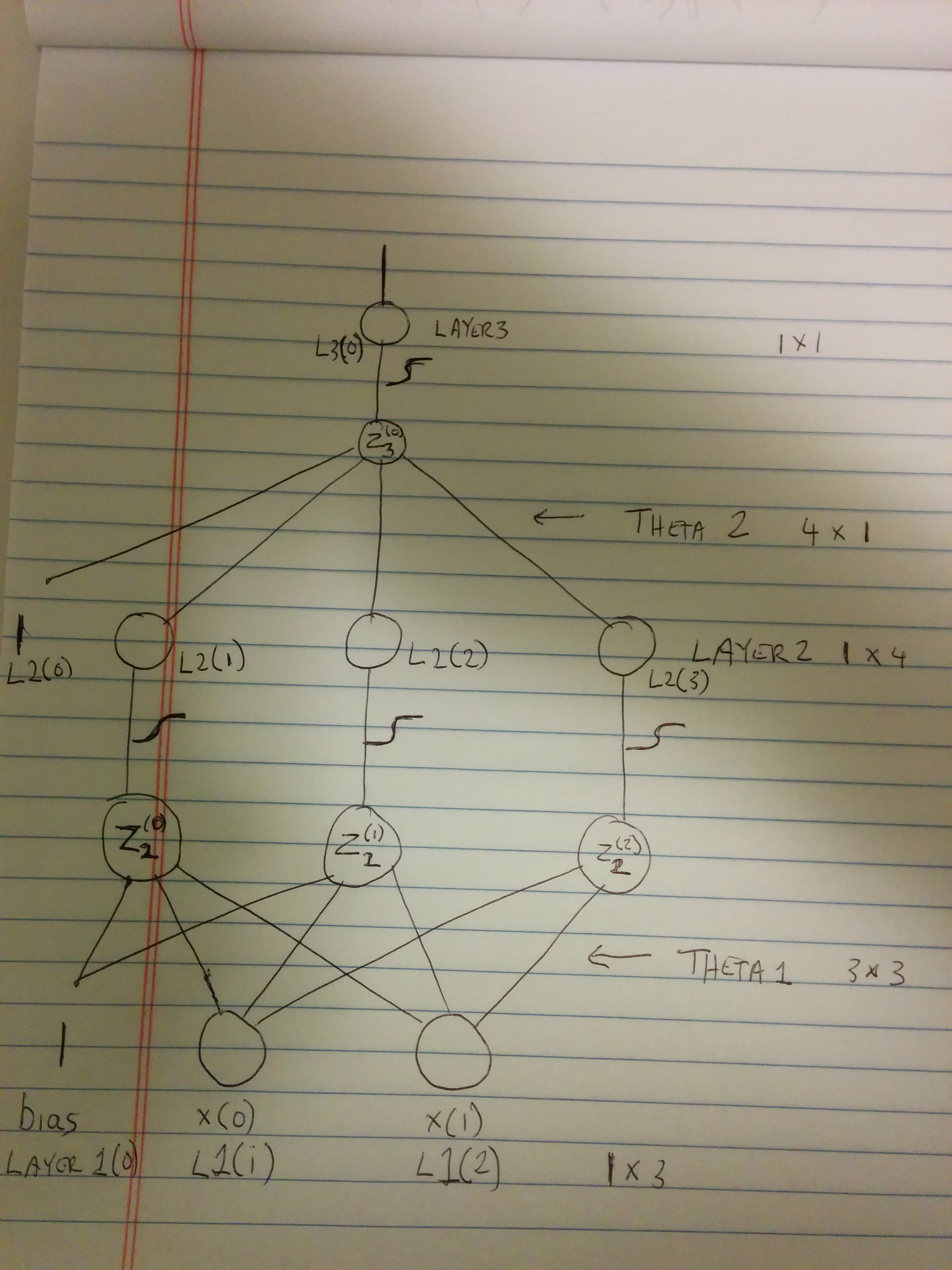
现在有一些解释。原谅原油画。拍摄照片比在gimp画画更容易。
Visual of WBC's xor neural network http://cablemodem.hex21.com/~binesh/WBC-XOR-nn-small.jpg
因此。首先,我们有错误功能。我们称之为CE(对于交叉熵。我会尝试尽可能使用你的变量,因此,我将使用L1,L2和L3而不是layer1,layer2和layer3。叹息(我不知道如何在这里做乳胶。它似乎在统计堆栈交换上工作。很奇怪。)
CE = -(Y log(L3) + (1-Y) log(1-L3))
我们需要获取此wrt L3的衍生物,以便我们可以看到如何移动L3以便减少此值。
dCE/dL3 = -((Y/L3) - (1-Y)/(1-L3))
        = -((Y(1-L3) - (1-Y)L3) / (L3(1-L3)))
        = -(((Y-Y*L3) - (L3-Y*L3)) / (L3(1-L3)))
        = -((Y-Y3*L3 + Y3*L3 - L3) / (L3(1-L3)))
        = -((Y-L3) / (L3(1-L3)))
        = ((L3-Y) / (L3(1-L3)))
很好,但实际上,我们不能只是改变我们认为合适的L3。 L3是Z3的函数(见我的图片)。
L3      = sigmoid(Z3)
dL3/dZ3 = L3(1-L3)
我不是在这里推导出来的,(sigmoid的衍生物),但实际上并不难以证明这一点。
但是,无论如何,这是L3 wrt Z3的衍生物,但我们想要CE的衍生物Z3。
dCE/dZ3 = (dCE/dL3) * (dL3/dZ3)
        = ((L3-Y)/(L3(1-L3)) * (L3(1-L3)) # Hey, look at that. The denominator gets cancelled out and
        = (L3-Y) # This is why in my comments I was saying what you are computing is the _negative_ derivative.
我们称衍生物为Z的“三角洲”。因此,在您的代码中,这对应于delta3。
很好,但我们不能随便改变Z3。我们需要计算它的衍生物,即L2。
但这更复杂。
Z3 = theta2(0) + theta2(1) * L2(1) + theta2(2) * L2(2) + theta2(3) * L2(3)
所以,我们需要采取偏导数。 L2(1),L2(2)和L2(3)
dZ3/dL2(1) = theta2(1)
dZ3/dL2(2) = theta2(2)
dZ3/dL2(3) = theta2(3)
请注意,偏见实际上是
dZ3/dBias = theta2(0)
但是偏见永远不会改变,它总是1,所以我们可以放心地忽略它。但是,我们的第2层包含偏见,因此我们暂时保留它。
但是,再次,我们想要衍生wrt Z2(0),Z2(1),Z2(2)(看起来我很糟糕,不幸的是。看看图表,它会更清楚,我想。)
dL2(1)/dZ2(0) = L2(1) * (1-L2(1))
dL2(2)/dZ2(1) = L2(2) * (1-L2(2))
dL2(3)/dZ2(2) = L2(3) * (1-L2(3))
现在是什么dCE / dZ2(0..2)
dCE/dZ2(0) = dCE/dZ3 * dZ3/dL2(1) * dL2(1)/dZ2(0)
           = (L3-Y)  * theta2(1)  * L2(1) * (1-L2(1))

dCE/dZ2(1) = dCE/dZ3 * dZ3/dL2(2) * dL2(2)/dZ2(1)
           = (L3-Y)  * theta2(2)  * L2(2) * (1-L2(2))

dCE/dZ2(2) = dCE/dZ3 * dZ3/dL2(3) * dL2(3)/dZ2(2)
           = (L3-Y)  * theta2(3)  * L2(3) * (1-L2(3))
但是,我们真的可以表达为(delta3 * Transpose [theta2])elemenwise乘以(L2 *(1-L2))(其中L2是向量)
这些是我们的delta2层。我删除它的第一个条目,因为正如我上面提到的,它对应于偏差的增量(我在图上标记了L2(0)。)
因此。现在,我们有Z的衍生品,但实际上,我们可以修改的只是我们的理论。
Z3 = theta2(0) + theta2(1) * L2(1) + theta2(2) * L2(2) + theta2(3) * L2(3)
dZ3/dtheta2(0) = 1
dZ3/dtheta2(1) = L2(1)
dZ3/dtheta2(2) = L2(2)
dZ3/dtheta2(3) = L2(3)
再一次,我们想要dCE / dtheta2(0)tho,这样就成了
dCE/dtheta2(0) = dCE/dZ3 * dZ3/dtheta2(0)
               = (L3-Y) * 1
dCE/dtheta2(1) = dCE/dZ3 * dZ3/dtheta2(1)
               = (L3-Y) * L2(1)
dCE/dtheta2(2) = dCE/dZ3 * dZ3/dtheta2(2)
               = (L3-Y) * L2(2)
dCE/dtheta2(3) = dCE/dZ3 * dZ3/dtheta2(3)
               = (L3-Y) * L2(3)
嗯,这只是np.dot(layer2.T,delta3),这就是我在theta2d中所拥有的
同样地: Z2(0)= theta1(0,0)+ theta1(1,0)* L1(1)+ theta1(2,0)* L1(2) dZ2(0)/ dtheta1(0,0)= 1 dZ2(0)/ dtheta1(1,0)= L1(1) dZ2(0)/ dtheta1(2,0)= L1(2)
Z2(1) = theta1(0,1) + theta1(1,1) * L1(1) + theta1(2,1) * L1(2)
dZ2(1)/dtheta1(0,1) = 1
dZ2(1)/dtheta1(1,1) = L1(1)
dZ2(1)/dtheta1(2,1) = L1(2)

Z2(2) = theta1(0,2) + theta1(1,2) * L1(1) + theta1(2,2) * L1(2)
dZ2(2)/dtheta1(0,2) = 1
dZ2(2)/dtheta1(1,2) = L1(1)
dZ2(2)/dtheta1(2,2) = L1(2)
并且,我们必须乘以dCE / dZ2(0),dCE / dZ2(1)和dCE / dZ2(2)(对于那里的三个组中的每个组。但是,如果你考虑这个,然后就变成了np.dot(layer1.T,delta2),这就是我在theta1d中所拥有的。
现在,因为您在代码中执行了Y-L3,所以将添加到theta1和theta2 ......但是,这是推理。我们刚才计算的是CE与权重的导数。因此,这意味着,增加权重将增加 CE。但是,我们真的想减少 CE ..所以,我们减去(通常)。但是,因为在你的代码中,你正在计算负导数,所以你添加它是正确的。
这有意义吗?